The MAX1463 is a fully digital, high-performance signal conditioner with multi-channel inputs. It has analog and digital outputs and supports 4-20mA output applications. It can be programmed to correct the nonlinearities and temperature-dependent characteristics of sensors.
This document describes the procedures to compensate and calibrate a sensor signal that is applied to one of the MAX1463 ADC channels, providing offset and span correction over the specified temperature range. It is assumed that the MAX1463 VDD supply voltage does not change during the compensation process and operation of the device.
The data presented in this document is real data, acquired from a piezoresistive pressure sensor that was used as an example to present the compensation algorithm.
Input Parameters
The user must define some input parameters for the application. They are:Tmin = minimum temperature, in degrees CelsiusThe next limits are application dependent, and may differ for other applications:
Tintr = intermediate temperature, in degrees Celsius
Tmax = maximum temperature, in degrees Celsius
Pmin = minimum pressure
Pmax = maximum pressure
Vmin = desired MAX1463 output, at the minimum pressure, in volts
Vmax = desired MAX1463 output, at the maximum pressure, in volts
For pressure nonlinearity correction, let's define Pmed as the sensor excitation midpoint, as:
For better performance and range of the MAX1463 ADC converter it is necessary to maximize its useful range by adjusting the appropriate coarse offset and PGA settings. The user must select the temperature for which the sensor sensitivity is the highest and apply minimum and maximum sensor excitation. The user should then select the PGA gain and coarse offset settings that maximize the ADC output at these conditions.
The ADC acquired data must then be entered in the matrix below. Each row of data has the normalized ADC reading for the minimum, medium and maximum sensor excitation at the indicated temperature. It also has the ADC reading for the internal MAX1463 temperature sensor, and the DAC output voltage (through either the small or large op-amp) for a fixed normalized digital input of -0.5 (DACinM) and +0.5 (DACinP)
The acquired data (ad) matrix is shown below, with the ADC results enteredin hexadecimal, and the DAC output voltage readings entered in decimal. Due to limitations of the software, hexadecimal values must be entered with a leading zero (0).
To convert the 2's complement hexadecimal values in decimal values (between -1 and +1), the following function is defined:
The decimal representation of the acquired data matrix is then defined as:
With the defined user values, the above matrix is shown as:
Let's define other parameters that will be used throughout the document:
Data Modeling
This section shows the mathematical data modeling of the sensor data, temperature data, and DAC data. The derived functions for the sensor, temperature, and DAC will then be used as their model.Sensor Data Modeling
For the sensor data modeling, we will first model the sensor data at each individual temperature. We will then model the variation of the coefficients over temperature. The coefficients are found solving a linear system of equations, described as:Ax = bwhere "A" is a square matrix, and "x" and "b" are column vectors.
x = A-1b
The inverse matrix, in this case, is defined as:
For the minimum temperature, the second order coefficients that model the variation of the ADC data over pressure are given by:
And the equation that models the ADC output over pressure at this temperature is given by:
For the intermediate temperature, the second order coefficients that model the variation of the ADC data over pressure are given by:
And the equation that models the ADC output over pressure at this temperature is given by:
For the maximum temperature, the second order coefficients that model the variation of the ADC data over pressure are given by:
And the equation that models the ADC output over pressure at this temperature is given by:
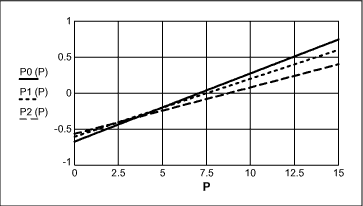
Figure 1. ADC output x sensor excitation (psi).
Now, let's combine these equations to include the temperature dependency. Basically, we will find second order equations that model the coefficients variation over temperature. The zero, first and second order coefficients on P0(T), P1(T) and P2(T) are given by:
For the temperature modeling of the coefficients, we now need to define the following matrix:
The zero order coefficients dependency over temperature can be found as follows:
And the zero order coefficient function is given by:
The first order coefficients dependency over temperature can be found as follows:
And the first order coefficient function is given by:
The second order coefficients dependency over temperature can be found as follows:
And the second order coefficient function is given by:
The ADC output, as a function of both temperature and pressure is then given by:
To verify the validity of the above equation, let's compare the data matrix with the values from the Pdata function.
Temperature Sensor Data Modeling
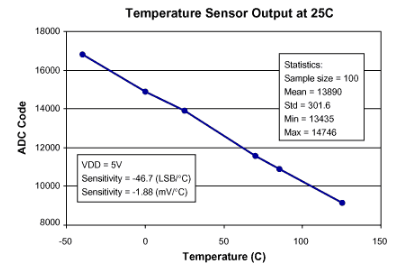
The internal MAX1463 temperature sensor must also be modeled. The ADCtemperature data was previously defined, and is given below:The second order temperature coefficients are then given by:
The temperature ADC output, as a function of temperature is then given by:
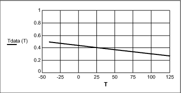
Figure 2. temperature ADC output x temperature(°C).
For verification, the values below show the input temperature data, and the values obtained from the Tdata function.
DAC Data Modeling
The MAX1463 DAC must also be modeled for properly adjusting its input values to the variations over temperature and process (gain, offset). The DAC data was already defined, and is given below, for both the Minus input (-0.5) and the Positive input (+0.5):The DAC gains for the input measured values are defined as:
The DAC offsets for the input measured values are defined as:
The coefficients of the second order function that represents the DAC gain over temperature are:
And the DAC gain function is then given by:
The coefficients of the second order function that represents the DAC offset over temperature are:
And the DAC offset function is then given by:
The final DAC characteristics can then be represented by:
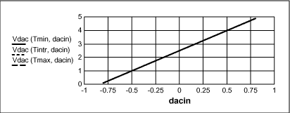
Figure 3.
For verification, the values below show the input DAC data, and the values obtained from the Vdac function.
Temperature Sensor Offset and Nonlinearity Correction
In order to minimize the temperature related coefficients, let's arrange the temperature characteristics, centering it at zero, and then amplifying it.To center the data points, the temperature data offset is defined as:
The offset corrected Tdata is then given by:
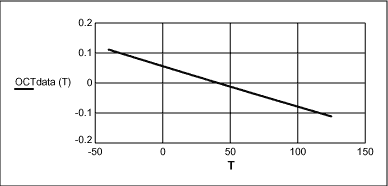
Figure 4. Offset corrected temperature data x temperature (°C).
The next step is to expand this function so that its minimum and maximum values are -0.9 and +0.9 (90% of the useful range). This is done to reduce the values of the temperature related coefficients that will be calculated in this algorithm. The temperature gain is given by:
As rtgain is outside the -1 to +1 values, it needs to be scaled down by a power of 2.
The final tgain is then: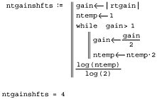
After multiplying tgain by OCTdata, the result needs to be scaled back up, shifting the result to the left (multiplying by powers of 2) by the same factor that was used in the downscaling process (ntgainshfts). Thefinal Amplified Offset Corrected Temperature data is then given by:
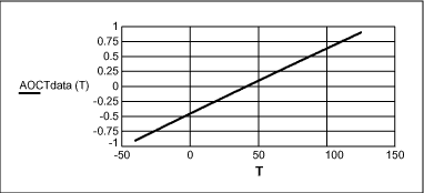
Figure 5. Amplified offset corrected temperature data x temperature (°C). where
The next step is the temperature nonlinearity correction. The linear coefficient of AOCTdata, using its endpoints, is calculated as:
And the nonlinear function can be expressed as:
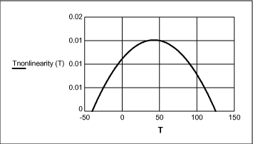
Figure 6. Nonlinearity of Temperature data x Temperature (°C).
We need to implement a function that represents the opposite of the nonlinearity function, using the AOCTdata(T) as the independent variable. As AOCTdata(T) is not linear, the best way is to use a fitting function to a higher order polynomial function. In this case, a fourth order polynomial function was chosen to minimize the nonlinearity errors.
The coefficients of the fourth order polynomial function are given by:
And the Temperature Nonlinearity correction function is given by:
The offset corrected and nonlinearity corrected temperature data is now given by:
From now on, all the temperature related coefficients will be calculated using Tempdata as the independent variable, as it is normalized and linear.
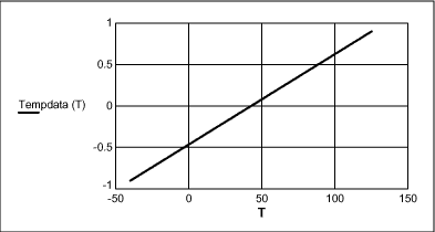
Figure 7. Linear temperature data x temperature.
The ideal temperature data is given by:
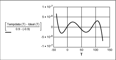
Figure 8. Linearity error of tempdata(T) x temperature (°C).
Sensor Signal Data Offset, Gain and Nonlinearity Correction
The sensor signal characteristics are also dependent on temperature and the excitation source (pressure). The objective here is to eliminate the temperature dependency and linearize the pressure response characteristics.Just as the case of the temperature signal, we will maximize the response to 90% of the total useful range, yielding -0.9 for minimum pressure, and +0.9 for the maximum pressure.
The raw sensor data is depicted below, for four different temperatures
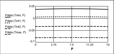
Figure 9. Raw sensor data x pressure (psi).
The linear coefficients for these curves, using the endpoint values, can be given by:
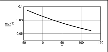
Figure 10. Sensor sensitivity x Temperature (°C). The pressure nonlinearity and offset correction function can be expressed by:

Figure 11. Sensor Offset and nonlinearity x Pressure (psi)
The objective now is to model the reciprocal of the pnl(T, P) function for four different temperatures, and then model the variation of the coefficients over temperature.
For the minimum temperature, the coefficients that approximate -pnl(Tmin, P) over a third order function of Pdata(Tmin,P) can be found by:
For the first intermediate temperature, the coefficients that approximate-pnl(Tint1, P) over a third order function of Pdata(Tint1,P) can be found by:

For the second intermediate temperature, the coefficients that approximate -pnl(Tint2, P) over a third order function of Pdata(Tint2,P) can be found by:
For the maximum temperature, the coefficients that approximate -pnl(Tmax, P) over a third order function of Pdata(Tmax, P) can be found by:
The matrix of correction coefficients for the calculated temperatures is given below:
The variation of those coefficients over the temperature data can be modeled by third order equations, solving a linear system:
The correction coefficients are:
And the zero, first, second and third order coefficient functions are given by:
The offset and nonlinearity correction function is then given by:
And the final offset and nonlinearity corrected sensor data is now given by:
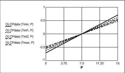
Figure 12. Offset and nonlinearity corrected sensor data x pressure (psi).
The next step is to remove the temperature dependency of the sensor sensitivity.
The span function over temperature is given by:
The sensitivity correction coefficients that approximate 1/span(T) over a 4th order function of Tempdata(T) can be found by:
And the sensitivity correction function can then be described by: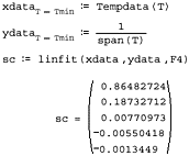
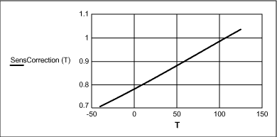
Figure 13. Sensitivity correction function x temperature (°C).
The corrected Sensor data is then given by:
The final data will be normalized to -0.9 for the minimum pressure and +0.9 for the maximum pressure. The normalization factor is given by:
And the final coefficients for the sensitivity correction function is then given by:
Where the normalized sensitivity correction function is given by:
The value of nSensC(T) has to be between -1 and +1 for the whole range of temperature. To ensure that this is true, we have to find the power of two divisor that scales back nSensC(T).
The final set of sensitivity correction coefficients is then given by:
And the final sensitivity correction function is then given by:
The final normalized corrected sensor data is then given by:
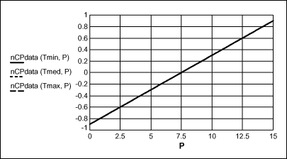
Figure 14. Normalized Corrected Sensor Data x Pressure (psi).
At this point, the sensor data is normalized to -0.9 to +0.9 for the minimum and maximum sensor excitation. All the nonlinearities have been corrected and the temperature dependency is removed. It is a very linear signal with respect to the excitation (pressure).
DAC Correction
This step is required to correct the nonlinearities and temperature dependency associated with the MAX1463 DACs, when an analog output is required. The minimum and maximum output voltages associated with the minimum and maximum sensor excitation were already defined, and are given by:The offset can then be defined as:
But the target offset value has to compensate for the DAC offset variation over temperature, which is given by:
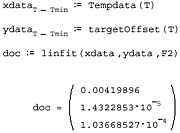
The dac offset correction coefficients that approximate targetOffset(T) over a second order function of Tempdata(T) can be found by:
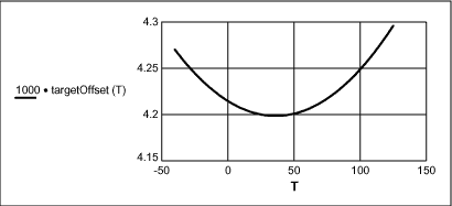
Figure 15. Target DAC input value x Temperature (°C).
And the DAC offset correction function can then be described by:
The DAC gain also has to be corrected for temperature variations. The function that corrects the DAC gain variations over temperature, and also adjusts the signals for the output span is given by:
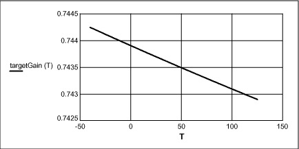
Figure 16. DAC gain correction x temperature (°C).
The dac gain correction coefficients that approximate targetGain(T) over a second order function of Tempdata(T) can be found by:
And the DAC gain correction function can then be described by:
The final DAC input, as a function of temperature and pressure, is then given by:
And the final DAC output over the sensor excitation (pressure) is shown below, for various temperatures.
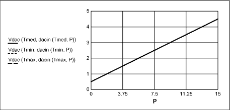
Figure 17. DAC output (V) x pressure (psi).
Compensation Coefficients and Equations
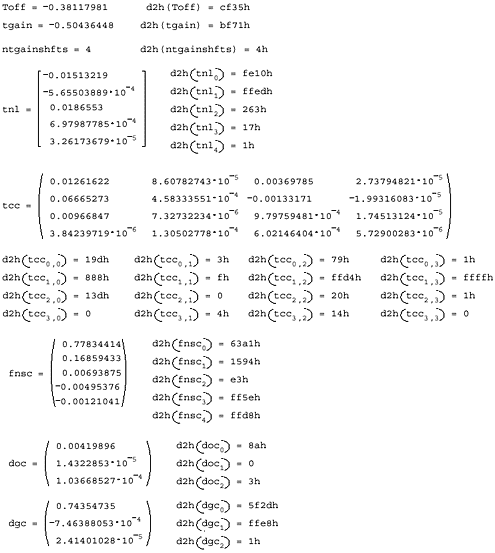
This section summarizes the compensation coefficients and equations that need to be implemented in the MAX1463. Note that the MAX1463 does not calculate the coefficients, as these need to be calculated using the algorithm described in this document.The temperature sensor data is shown as Tdata(T), and is the result of the ADC conversion of the internal MAX1463 temperature sensor. The sensor data is shown as Pdata(T), and is the result of the ADC conversion of the sensor signal.
The program needs both the temperature sensor data, and the sensor signal data. As the temperature rate of change is much slower than the sensor signal data, the user can decide to do a temperature ADC conversion on a much slower rate than the sensor signal, typically once every few hundred sensor signal conversions.
The following functions are defined to convert the calculated coefficients to a two's complement hexadecimal representation. Note that the digitized coefficients may differ from the calculated ones due to quantization on a 16-bit level.
Compensation Coefficients
Temperature Loop Compensation Equations
The following set of equations provide correction on the MAX1463 Temperature Sensor data.The next set of equations provide correction on the sensor signal data.

The next set of coefficients and equations provide correction on the MAX1463 DAC data.

Sensor Signal Loop Compensation Equations
The following set of equations provide correction on the MAX1463 Pressure Sensor data.
At this point, just write the final result, dacin(T,P) to the DAC input to obtain the compensated output, and return to the beginning of the sensor signal loop. The user may implement a counter to keep track of the number of sensor signal conversions, and do a temperature loop every so often.
 電子發(fā)燒友App











評(píng)論